Introduction
The goal of this project was to build a profitability model based on total spirits sales in Iowa at the store level. Since it is a very large data set, only 10% of the data was retrieved from the Iowa website. The dataset contains the spirits purchase information of Iowa Class “E” liquor licensees (stores) by product and date of purchase from the state of Iowa. For the variables’ description, please visit the Iowa website.
Note the data does not contain total sale of liquor for each transaction made by customers in each store. Instead, it contains total sale of liquor per transaction made by each store while purchasing liquor from the state of Iowa. Thus, while exploring the data, a very important assumption was made that owners in Iowa are knowledgeable business people, and they only stock what they sell. In addition to the variables I had, three new variables were created: Store (a number of stores per each zip code), Vendor (a number of vendors per each zip code), and Month (a month when liquor was purchased).
Multiple Regression Model
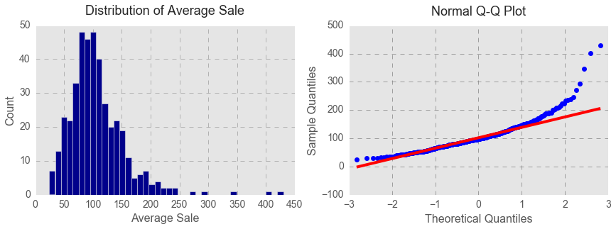
Since the outcome variable Sale is continuous, a multiple regression model was built. I used a stepwise approach in building the regression model. However, first and foremost, I looked at average sales per transaction that are outliers. As seen below from the histogram and Q-Q plot, average costs per transaction that exceeded $250 were exceptions.
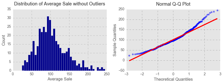
After removing the outliers, the distribution of average cost per transaction looked much closer to normal distribution.
Finally, I got to conduct a stepwise regression to select my final linear regression model. Stepwise regression is a method of fitting regression models step-by-step. In each step, I consider a variable to add to or subtract from the set of all variables based on an adjusted R-squared. If I saw no changes in an adjusted R-squared, I would not include that variable into the statistical model. I also looked at multicollearity. The highly correlated independent variables were removed from the model.
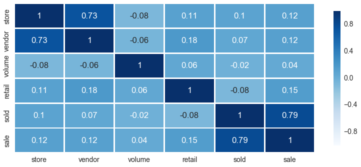
I excluded variable Cost (cost per transaction) as it was highly correlated with Retail (retail price per transaction). Because Store (a number of stores per each zip code) and Vendor (a number of vendors per each zip code) were highly correlated (r=.73), I also removed Store out of my model. Additionally, I checked whether Store affected in anyway the adjusted R-squared and found no changes there.
Since the variable Month did not predict Sale, the final model excluded the month when liquor was purchased. Consequently, I adjusted density of the data points by removing the variable Month from my data.
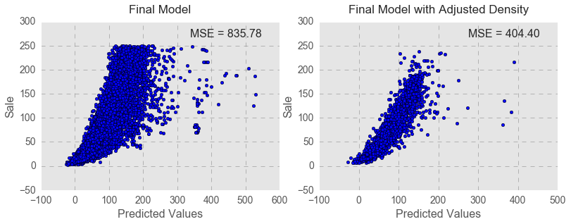
After regrouping the data, MSE (mean squared error) of the final regression model substantially decreased (404.40 vs. 835.78).
As seen in the regression table below, all independent variables positively and significantly predicted average sale per transaction. Sale per transaction increased as Retail (retail price per bottle), Sold (a number of bottles sold), Vendor (a number of vendors per zip code), and Volume (bottle volume) increased. All categories of liquor (except schnapps) significantly predicted sale per transaction compared to brandy (the baseline category).
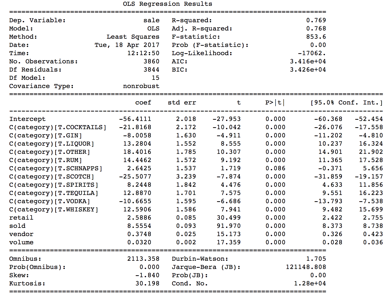
The scatter plot and OLS line for predictions vs. average sale per transaction demonstrates the final regression model by liquor category. The model yielded adjusted R-squared of .768 and MSE of 404.40.
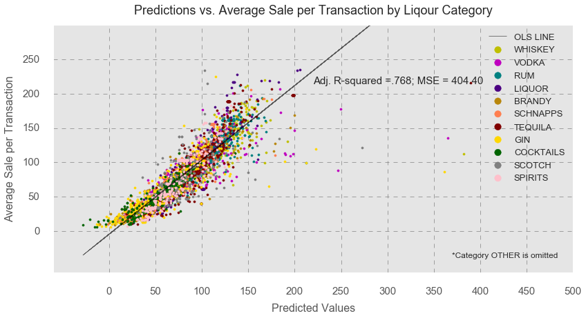
Liquor, whiskey, vodka, tequila, and schnapps had the highest average sale per transaction, indicating that these types of liquor are more likely to sell compared to the other types of liquor.
Assumptions of Linear Regression
Before finalizing the model, I checked whether it meets 4 linear regression assumptions: 1) linearity and additivity of the relationship between dependent and independent variables, 2) statistical independence of the errors, 3) normality of the error distribution, and 4) homoscedasticity (constant variance) of the errors.
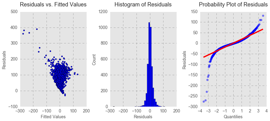
As the scatter plot above indicates, there is a linear relationship between predicted values and sale. The Durbin – Watson (DW) statistics in the table above indicate that the regression model has a very slight positive autocorrelation with DW =1.70, but this value is also not large enough to discard the model. Thus, we can say that the final regression model met the assumptions of linearity and statistical independence. The probability plot of residuals and the histogram of residuals demonstrates no indication of abnormal distribution of errors. However, the residuals vs. fitted values plot obviously signals the presence of homoscedasticity as indicated by the funnel shape of the scatter points.
Nonparametric Approach
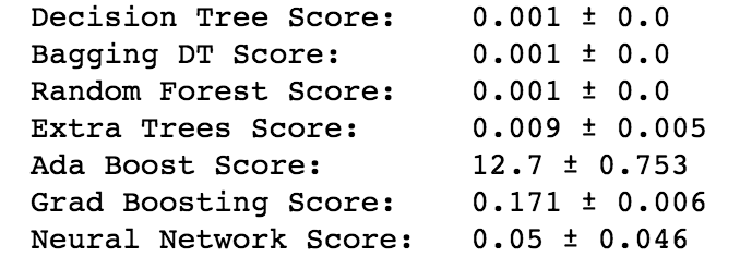
Since the final regression model did not meet the assumptions of homoscedasticity and barely met the assumptions of linearity and statistical independence, it could not be used as a final profitability model for Iowa liquor stores. Instead, I ran and cross-validated several non-parametric repressors: Decision Tree, Bagging DT, Random Forest, Ada Boost, Gradient Boosting, and Neural Network. I used MSE as a cross-validation score, and there were some fluctuations in the scores. As seen below, Ada Boost algorithm yielded slightly lower accuracy score on the training set than the other algorithms, as indicated by higher MSE.
I chose the Decision Tree regressor and Ada Boost regressor as my final non-parametric profitability models. The decision tree model was one of my choices because in spite of its propensity to overfitting, it is the easiest model to use and interpret (after the linear regression), performs well with a large set of data, has a higher training and prediction speed.
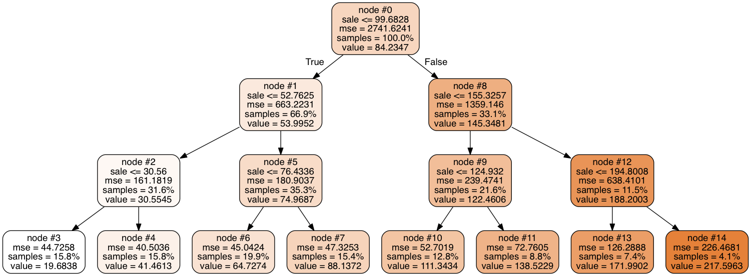
As seen above, the decision tree regressor builds a regression model in the form of a tree structure. Here, I am only presenting a tree with a maximum depth of 3, for a demonstration. A decision node Sales has two original branches, sales that are equal to or more than 52.76 and sales that are equal to or more than 155.33, each representing values for the attribute the attribute tested. A measure of purity is calculated for each branch, which represents the amount of information needed to classify instance as True or False. The branches split into smaller successively purer subsets further and further until they reach the best possible purity.
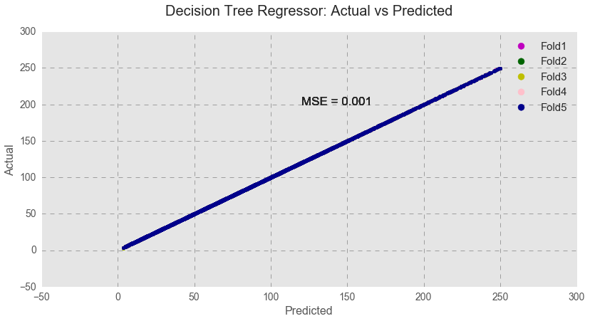
However, as seen below, the decision tree model perfectly fits the test data over 5 folds, and I am very suspicious that it might be a sign of overfitting.
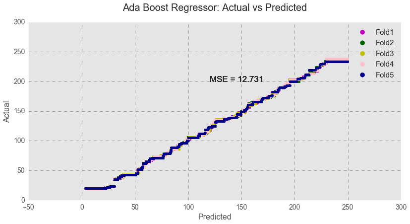
The Ada Boost algorithm is more robust to overfitting and yields more accurate results, but is much harder to interpret. Indeed, Ada Boost yielded a slightly higher MSE score, indicating a slightly lower accuracy. Even so, the algorithm with the lower accuracy might be an equally good choice in this case in order to avoid the model’s overfitting. As shown below, testing data over 5 folds produced a zigzag-like pattern, indicating a slightly lower model fit.
Since both non-parametric models have their advantages and disadvantages, it is hard to say which one is better. I would keep both machine learning algorithms for future evaluations and apply them both to new data sets to evaluate the model’s accuracy.
Conclusion
In this project, I built a profitability model for Iowa liquor stores. First, a linear regression model was constructed using a step-wise approach. However, the model did not meet all the linear regression assumptions, and I had to use non-parametric algorithms. I ran six algorithms and all of them (except Ada Boost) produced similar accuracy scores as measured by MSE. Because the scores were close to prefect, possibly indicating an overfitting, I selected Ada Boost (along with Decision Tree) as my final algorithms. Ada Boost is very hard to interpret but more robust to overfitting. Decision Tree, on the other hand, is easy to interpret, performs really well with a large set of data, has a high training and prediction speed, but is prone to overfitting.
